Algebra
This is an online resource for instructors and students. While the material is designed to be taught to strong middle school students, these notes are written for instructors who are invited to guide and discuss topics with their students.
- Algebra
- Fundamentals
- Rational Numbers
- Linear Equations
- Real Numbers
- Polynomials
- Linear Algebra
Fundamentals
The Integers
The first kinds of numbers discovered were the natural numbers:
There are (infinitely) many natural numbers, and there are many things that we can do with them. For example, we can add any two natural numbers to obtain another. It does not matter how big the numbers become: their sum is always still a natural number.
We may also multiply two natural numbers to obtain another. Again, it does not matter how big or small the numbers are: multiplication is something we can do with any natural numbers.
Natural numbers are great for representing “things”. In particular, they're great for representing “some number of things”. But they fall short when we want to represent less than nothing. But you can’t have less than nothing, so why would we ever want that?
The desire for a more general kind of number comes from the desire to represent change. If yesterday there were students in attendance, and today there are students in attendance, then we can say more people attended today than did yesterday. But what if tomorrow there will again be students in attendance? Then how many more students will have attended? Even worse, what if the day after tomorrow, there will be students in attendance again. Then what is the change in the number of students?
It is not that these problems cannot be solved with positive natural numbers. In fact, they certainly can. The number of students could increase by , and we have a number for that. Or the number of students could decrease by . We already have a number for that.
So to express a change in a quantity, we must convey two pieces of information: firstly, in what direction is the change; and secondly, by how much the quantity is changed. This seems quite complicated. It would be simpler to introduce a new kind of quantity that could represent these changes more conveniently and more compactly. This, of course, is the motivation for negative numbers.
Negative numbers do not “exist” in the real world. We cannot have a negative number of people in a class. But they provide an easy way to talk about change: if positive numbers represent increase, then negative numbers represent decrease.
The introduction of negative numbers allows us to expand our set of mathematical objects to the integers, . As with natural numbers, we still have these two useful properties of integers, which we will call closure properties (think of a room withh closed door; if applying these operations inside the room of the integers, you never need to worry about anything outside the room):
The sum of any two integers is again an integer.
The product of any two integers is again an integer.
But in addition, we have a third closure property, which enables us to describe changes:
The difference of any two integers is again an integer.
Variables
When we first learn arithmetic, we only have to worry about natural numbers. As we continue to develop new techniques, we find new kinds of numbers — like the integers mentioned above. Let’s take a step back and examine the philosophy behind what numbers really are.
We are familiar with everyday objects: things we can see, feel, or otherwise interact with. Mathematical objects are like those, but more abstract. In the mathematical world, you can interact with mathematical objects through statements of fact. A common example of such a statement is equality: is a statement of fact that the mathematical object referred to by is in fact the same as the mathematical object referred to by .
Numbers are the most common mathematical objects, but as we will see later, they are not the only kind. Typically, we study mathematical objects because of some motivation from a real-world problem. In the real world, we may talk of quantity, location, a process, or any number of other things. To use mathematics to solve these problems, we must translate these real-world concepts into mathematical objects by using a model. Inside the model, we have many mathematical objects. Some of these objects represent the information given to us by the problem. Other objects might represent information we need to figure out — they might not be known from the start!
There are three ways we can describe a mathematical object in a simple model:
A literal: for example, just a number, like .
A variable: a letter that we understand the meaning of, but we may or may not know the value of, like . Essentially, we are naming a mathematical object. It can sometimes be useful to name known objects (for example, if they are complicated), but usually we only use variables for unknown objects.
An expression: a combination of literals, variables, and operations, like .
For instance, a real world problem is as follows:
Exercise 2: More Lumber Is Required
Yahui and Zhen want to build a wooden treehouse. planks are required. Yahui has in her shed, and Zhen has in his shed. How many additional planks must they buy to complete the treehouse?
Solution
We can use whole numbers to model this problem. First, let’s give names (variables) to all mathematical objects (numbers) that the problem gives us or requests that we find. Let be the number of planks that Yahui has, be the number of planks that Zhen has, be the total number of planks required, and be the number of additional planks they must buy. The equation is:
This equation is the governing equation of our model. We are given the values of , , and , and we’re asked to find the value of . (This is not always possible!) As mentioned above, we don’t need to use names for the known values, so we can substitute the literals:
To find the unknown value we must add to to arrive at , we can use subtraction. That is,
Another way to understand what we have done in the above step is that and refer to the same mathematical object, . Therefore, we can subtract from both of them, and they will still be different names for the same object. That is, . By using the properties of addition that we are familiar with, the left hand side is just another name for — and so we obtain the result seen above.
In this example, all of the variables we used represent specific mathematical objects. Three of them were immediately given to us in the question. The other, , still represented a specific mathematical object, but we had to figure it out.
It is not always the case that variables represent specific mathematical objects — sometimes, we can attach a quantifier to a variable, to say that a statement is true of all mathematical objects of a certain type at once.
Exercise 3: Properties of Whole Number Addition
Give a concrete example for each of the following properties of addition of whole numbers:
For all integers , .
For all integers and , .
For all integers , and , .
Note that these concrete examples are applications of, not justifications for, the properties in question. It can be difficult to give a formal justification for true properties that involve quantifiers. However, if a statement is false, it is often much easier: we can simply give a single concrete example which does not satisfy the statement.
Exercise 4: Counterexamples
Give a counterexample for each of the following incorrect statements about whole numbers:
For all integers , .
For all integers and , .
For all integers , and , .
Note that even though each of the statements is false, they all have certain cases where they do hold. In the future, we will see techniques to find out exactly which cases the statement is true in.
Rational Numbers
The motivation behind fractions is similar to that of expanding the whole numbers to the integers. Many things in the real world are divisible into portions. For instance, we can cut a cake into slices. Natural numbers are good at counting wholes, but bad at measuring parts of wholes.
To solve this problem, we introduce the concept of splitting a single whole into equal parts, where is a positive whole number. (Later, we will allow to be negative, but it cannot be zero — it is not possible to split something into zero equal parts.) We write this as , and call each of the equal parts an th part. (If , then they are called tenths.) We may sometimes require more than one such equal part. If we want parts where is any integer, we will write it as .
All numbers that can be formed from fractions of integers are called rational numbers. We can talk about rational numbers as an extension to the integers, just like how we did with integers above, as an extension to the natural numbers. Each integer is still a rational number: for every integer , and .
There are various simple properties of fraction addition and subtraction, and multiplication, by counting the number of of th parts:
For all integers , , and , if , then .
For all integers , , and , if , then .
For all integers , , and , if , then .
With the integers, we could not in general perform exact division on any two integers. Fractions cover the case of dividing almost any two integers (almost, since the denominator may not be ). But do we still have closure under addition, subtraction, and multiplication? Moreover, do we almost have closure under division (if we disallow a zero divisor)? We only saw some special cases of these operations above. We need to introduce stronger techniques — a general way to do addition, subtraction, and multiplication of fractions, to show that this closure is indeed the case.
Fraction Multiplication
We saw above how to multiply a fraction by an integer. This has the same meaning as multiplying two integers; we can think of it as adding (maybe in the negative direction) repeated copies of the fraction. But it is harder to extend this idea toward multiplying two fractions: what do we mean when we say we want copies of ?
Luckily, there is in fact a single reasonable meaning for this. Recall that means to split a single whole into equal th parts, then take copies of the th parts. We can replace the single whole with something that is itself an arbitrary rational number: let mean to split into th parts, and then take of those. Then, , as we would expect.
How do we split into th parts? We can split each of the copies of the th parts into parts, then only take one of every . Each small part is a th part split further into parts. In a single whole, there would be equal such parts, so these small parts are in fact each.
Therefore, we can justify the following fact (or definition, or a sort) about fraction multiplication:
Fact 1: Fraction Multiplication
Let , , and be integers with . Then
Equivalence Classes
It happens to be the case with fractions that distinct ordered pairs might represent the same quantity. For instance, and are different pairs of numbers, but they represent the same fraction: one half. All the fractions that represent the same particular quantity form a so-called equivalence class. In a sense, this is not very different from and representing the same change in quantity .
How can we decide whether two fractions represent the same quantity? That is, suppose that and are rational numbers. Are they equal? In the case where the denominator is the same, this is easy to answer: just compare the numerators. Rational numbers with the same denominator are equal if and only if the numerators are equal.
Fact 2: Equivalence of Fractions With Equal Denominator
Let , , and be integers, and . Then
If the denominators are not the same, we need to rewrite the two fractions to have the same denominator. We can do this by first noticing the following fact, which we can obtain from our knowledge of fraction multiplication:
Fact 3: Common Factor of Numerator and Denominator
Let , and be integers, and . Then
This fact allows us to rewrite as , and as . Now the denominators are the same (remember for any integers and ). So we can simply compare with !
Visually, we are multiplying the top-left with the bottom-right, and the top-right with the bottom-left. This makes a cross shape, so one way to remember this technique is that it is often called “cross-multiplication”.
Fact 4: Cross-multiplication
Let , , and be integers, and . Then
Addition and Subtraction
We have seen above the example of rewriting fractions with a common denominator in order to compare them. But another use of fractions with a common denominator is that they are easy to add and subtract. We can apply the same technique:
Exercise 5: Fraction Addition and Subtraction
Rewrite the fractions using a common denominator in order to calculate:
In general, we can derive formulas for addition and subtraction of fractions, but you should not memorize them. It is more useful to understand the process of arriving at the formulas.
Fact 5: Fraction Addition & Subtraction
Let , , and be integers with . Then and
Notice the resemblance to cross-multiplication. This is not accidental! From the subtraction formula, we see that if two fractions are equal, their difference is zero, and vice versa.
Simplification
Often, given some fraction, we want to find the equivalent fraction with the smallest possible positive integer denominator. This is called the simplest form and is is useful for various reasons:
Smaller positive integer denominators are easier for people to understand.
Two fractions that are equal will have the same simplest form, so fractions in simplest form are easy to compare.
Reducing a fraction to simplest form is a matter of finding the largest common factor of both the numerator and denominator, and then dividing both the numerator and denominator by it.
Exercise 6: Fraction Operations and Simplification
Compute each of the following, then reduce it to simplest form.
Exercise 7: A Telescoping Product
Compute and reduce to simplest form:
Solution
Each fraction in this product, except for the last one, has a numerator which is the same as the denominator of the following fraction. These will cancel out if we multiply the fractions. For instance, , and we can divide from both the numerator and the denominator to get .
In this manner, all the numbers except for the first in the numerator and the last in the denominator will get cancelled out. So we are left with .
Linear Equations
Ratios and Rates
Frequently, we may know certain quantities not in absolute terms, but only in relative terms. What does this mean? Let’s say you see two weights on the ground, labeled A and B. You might notice that B is twice as hard to lift up as A. Without a scale, it is hard for you to measure the actual weight of the objects, but you might be able to estimate the ratio of their weights.
In another example, suppose you are counting cars as they pass by on a highway. You might notice that for every personal cars you count, you see about one truck. It might be hard for you to estimate how many cars are passing by each minute, since it is hard to guess how long a minute is, but you could estimate the ratio of personal cars to trucks on this highway.
We will see a couple of word problems that involve known ratios, and try to determine the absolute quantities using additional information provided to us.
Exercise 8: Carcross Car Count
The community of Carcross, Yukon is quite small, with a population of only 301. Caroline counts the number of cars that passed her house over an hour and noticed that:
There were cars that passed in total.
All cars were either blue or silver.
Twice as many cars were blue than silver.
How many blue cars passed by? How many silver cars?
Solution
Let and be integers representing the number of cars that passed her house. Then our equations are:
We can substitute the second equation into the first equation, since and refer to the same mathematical object. Thus: so there were silver cars. Then we can substitute this back into that second equation . So , and so . Therefore there were blue cars.
Exercise 9: Produce Price Sum
A supermarket stocks four kinds of produce: apples, oranges, tomatos, and potatos. Apples cost twice as much as oranges, and oranges cost twice as much as tomatos. August bought of each kind of produce, and the total price was .
Can we figure out what was the price of tomatos? If so, what was it?
Solution
Let , , , and be rational numbers representing the prices of apples, oranges, tomatos, and potatos, all in dollars per kilogram. Then our equations are
If we substitute the first and second equations into the third, we get and thus . But there is a problem: there are multiple solutions to this! There are even multiple integer solutions; for instance, maybe and , or and . So we do not have enough information to figure out the price of tomatos.
Exercise 10: An Unlikely Sprint?
Miran, Gosse, and Brayan participated in a sprint. Miran tells you that she won and was twice as fast as Brayan. Gosse agrees that Miran won, and says he was close behind with a time only higher than Miran’s. Brayan says that he came in last with a time longer than Gosse’s time.
You know, however, that sometimes Miran, Gosse, and Brayan aren’t the most reliable. Is it mathematically possible for all of these accounts to be accurate? If so, do we have enough information to determine what were each of their times? If so, calculate the times.
Solution
Let denote Miran’s time, denote Gosse’s time, and denote Brayan’s time. Based on what everyone said, the equations are:
Substitute the expression for given by first equation into the second equation, to get
Now substitute this into the third equation, to get
We can now substitute this back into to get , and into to get (very fast indeed, maybe suspiciously so!).
We can check that these times match all three of the equations above, so it is mathematically possible and unique. This doesn’t mean that the statements were accurate, but they are not mathematically contradictory.
Exercise 11: Raccoon Population Growth
The number of raccoons in the city of Raccoonville is plotted on the following chart:
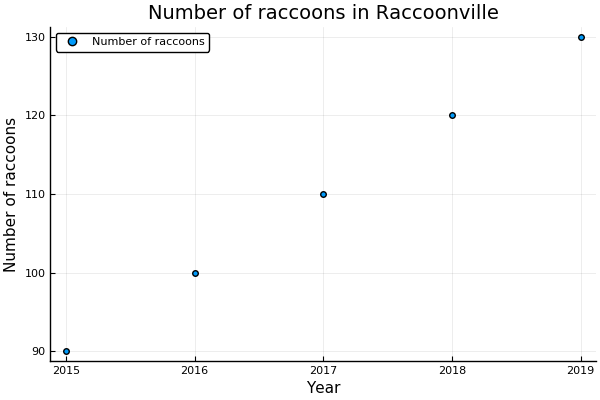
If the current trend continues, by what year will there be 180 raccoons in Raccoonville?
Solution
In this problem, we have to figure out the rate of increase of raccoons from the chart. The trend seems to be a straight line with an increase of raccoons every year. We can assume this trend will continue as the question asks us in that hypothetical. Let denote the number of years after . Then the number of raccoons will be . We want to solve:
Since this means years after , the year that there will be raccoons in Raccoonville is .
A General Approach
The examples above all have the same general form, where we have a number of equations of the form , where , , and are rational numbers, and we know and (but not ). Equations of this form are called “linear equations”. Why are they linear? Intuitively, one reason is that if we draw a line graph of the value of as we increase the value of , we will find a straight line:
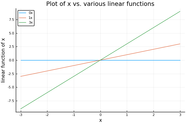
The solution to , if one exists, is simply where this straight line reaches a vertical height of . We saw a general technique to do this if : we can multiply both sides by (or equivalently, divide both sides by ). Thus the solution is .
But what if ? In this case, we cannot divide by , since division by is meaningless. Instead, we have the flat blue line in the graph. Obviously, this line will never reach any vertical height except ! Therefore, there is no solution if . If , then we still have no information about : any rational number will do. In this case, there are multiple solutions.
Real Numbers
Exponents
Recall that a positive exponent represents repeated multiplication, much like how a positive multiplier represents repeated addition. We can express this rule recursively using the following identity: which says that if you increase the exponent by it is the same as multiply one more copy of the base.
Exercise 12: Positive Integer Exponents
Evaluate each expression. Write your answer as an integer in literal form.
There are a variety of facts about positive integer exponents that we can justify using the properties of multiplication. Here are a few. You do not need to memorize these, but it is helpful to understand why they are true.
Fact 6: Sum of Exponents
If is a rational number, and and are positive integers, then . That is:
(Notice how when , this is just the recursive rule we discussed above.)
Fact 7: Product of Exponents
If is a rational number, and and are positive integers, then . That is:
It is frequently useful to extend the system of exponents to non-positive numbers, which can be done by applying the recursive rule in the other direction. Thus we can derive that and that for all non-zero values of . We can check that this extension retains the sum and product rules of exponents that we mentioned above, which is a useful feature.
Exercise 13: Negative and Zero Exponents
Evaluate each expression. Write your answer in simplest form as a fraction or as an integer literal.
A useful application of exponents is in shrinking large numbers to an more humanly understandable format. Indeed, we have a poor conception of how large certain numbers are. In science, it's common to see numbers way too large to count or way too small to visualize. Scientists have developed notation using exponents to make comparing such numbers easier. In scientific notation, a number is written as , where is a number with exactly one non-zero decimal digit before the decimal point, and is a (positive, negative, or zero) exponent.
A natural question to ask after having defined negative exponents is: what about rational exponents? Could those be useful? In fact, for a positive rational number base, we may sometimes define rational exponents in a way that preserves both the sum and product laws of exponents mentioned above. The only way to do this is to ensure that , that is, must be the th root of . We can also write that as . With this definition and the product law, we can define for any positive rational base and any rational exponent .
Exercise 15: Fractions, Exponents & Radicals
Evaluate each expression. Write your answer in simplest form as a fraction, or as an integer using the place value system.
With integer exponents of rational numbers, we are always guaranteed that the result exists and is a rational number (since we compute these exponents by multiplying and dividing rational numbers, which are closed under these operations). As we will see later, when rational exponents are concerned, the result may not exist as a rational number.
Definition of a Real Number
In previous sections, we were careful to only discuss square roots and other rational exponents when we knew that there was in fact a rational number that worked. In general, we cannot assume this is always the case.
We can give a proof that no rational number is equal to . One way to see this is a so-called proof by contradiction. In this kind of argument, we assume that is in fact rational. That is, if for some integers and in simplest form, then , so . We see that is a factor of the right hand side, so it must also be a factor of the left hand side. But the left hand side is a square, so for some integer . Then so . Now is a factor of the left hand side, so it should also be a factor of the right hand side. But the right hand side is a square, so for some integer . But then is clearly not in simplest form, so we have reached an absurd state — a contradiction. But of course, this is not possible, so something has gone wrong. Our argument is correct, so it must be our assumption that was wrong. The assumption we made was that is a rational number.
Many of you will probably be uneasy with how we are talking about as if it must exist, when we have already shown that no rational number squares to . We have already complicated things by introducing fractions to the easier world of the integers! If we make the claim that should exist as a number, then we run the risk of making things even more complicated and difficult. We don’t, in general, say that everything which doesn’t exist must be a new kind of number (we are happy to say that simply does not exist).
There is in fact a good reason, however, to suggest that might be a useful number to have. The reason for this is that we can already get very very close to a potential square root of ! An example of this is the rational number . In fact, we can get arbitrarily close. A way to visualize this is to see a graph that maps numbers to their squares.
We can start by plotting a point on some axes for integer values. The horizontal distance represents the number , which we vary to take on the integer values we want to show. The vertical distance represents the square of that number, .
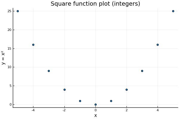
Of course, we can also take the square of rational numbers. We can think of this as increasing the precision of our graph by plotting more points, for example, every .
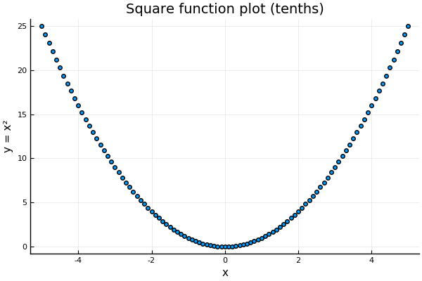
If we imagine that we continue this process, getting more and more precision, we would expect this curve to become continuous. We can see that it reaches a vertical value of at some point, and we saw earlier that no such rational number point exists. But the curve suggests that we can define a new kind of number that is on the number line, and we can get close to using rational numbers, but can’t get exactly there. This concept is called a real number.
There are many ways to formally define a real number, but it is not necessary to understand such a definition to understand what a real number is. Intuitively, we expect real numbers to plug the holes in continuous lines that we can draw. We can get as close as we want to a real number using rational numbers. In fact we don’t even need to use all rational numbers. All finite decimals are rational numbers, and by adding more decimal points, we can get closer and closer to any rereal number we are interested in. , but an even better approximation is . We can keep getting more and more precise, but we can never reach the number itself because it is not rational (hence not a decimal).
Operations on Real Numbers
We are able to add, subtract, multiply, and divide (except by zero) real numbers, just as we can with rational numbers. (Remember that we can get as close as we want to a real number using rational numbers. So it makes sense that real numbers behave almost identically to rational numbers!)
However, unlike rational numbers, it is not always possible to write real numbers in a canonical simplest form. Instead, we can use algebraic techniques to make expressions look simpler from a human perspective.
Exercise 16: A Linear Equation using Real Numbers
Solve the following equation for real number :
At this stage, it is helpful to understand some supplementary material on sets. This material is on a seperate page because it is not strictly related to what we are studying right now about algebra, but the notational conveniences of the material will be useful.
Polynomials
Linear Equations, Again
Recall earlier when we solved linear equations of the form , where and are known rational (or real) numbers, and is an unknown rational (or real) number. The solution is to divide both sides of the equation by , which is valid because and are different names for the same rational (or real) number. This results in the solution .
Note that many equations that may look different are really linear equations after some rearranging. For example, can be rearranged into the linear equation . can be rearranged into the linear equation . We will say that a linear equation that looks like is in “standard form”.
Let’s now look at a graphical method to solve a linear equation in standard form. What we will do is rewrite the right hand of the equation from to another variable . We will then draw a graph, similar to what we did earlier when we introduced real numbers. Let us first consider the linear equation .
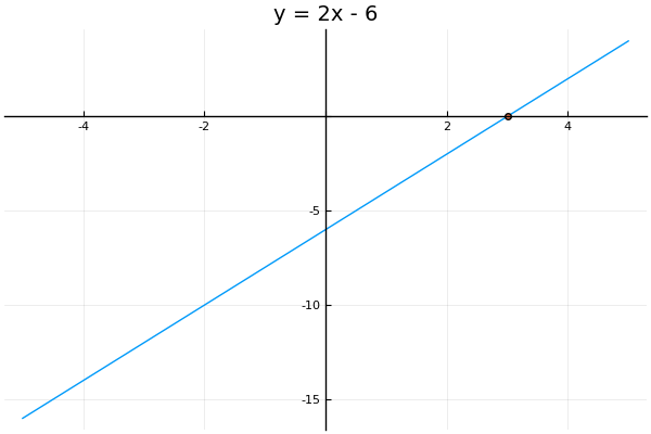
Note that the equation is more general than . If we set , then we get back the original equation . Therefore, to solve this equation we can look on the graphical plot for all the values on the line corresponding to . We see that this is where the line intersects with the x-axis. This is called an x-intercept, or root, of the function . From the plot, we see that the only root is , which corresponds to the only solution to this equation.
Two Simple Quadratics
We will now use the knowledge about plots and roots to solve equations which are not linear. Let us start with a simple example.
Exercise 17: Roots of
Plot , determine its roots, and use this information to solve the equation .
Solution
Here is our plot:
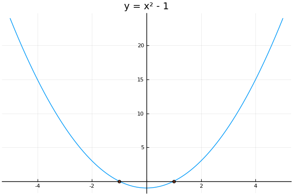
The roots are marked. They are and , which correspond to the solutions to our equation .
Exercise 18: Roots of
Without using a plot, determine the roots of . These are also solutions to the standard form equation ; explain why.
Solution
The roots occur when , so we want to solve . If the product of two numbers is , that means either the first number is or the second number is (or both). Therefore, the set of solutions to the equation is the union of the set of solutions to and the set of solutions to . If , this is a simple linear equation, where is the only solution. If , this is also a simple linear equation, where is the only solution.
Therefore, the roots are .
Note that by using the distributive property, we find that . So in fact, for all values of . Hence the solutions of the two equations must be the same!
Exercise 18 suggests a general approach to solving equations that involve and might be to decompose it into the product of two components which are both linear. This process is called factoring. An expression of the form , where , , and are known, is called a quadratic polynomial, just as where and are known is called a linear polynomial.
Factoring Quadratics
Suppose we have , where , , , and are known real numbers with . Then we know the solutions are . A quadratic polynomial written this way is easy to solve! Our goal is to take a polynomial in standard form, and convert it into this factored form.
It is easier to go backwards. From factored form, we can use distributivity to expand: . But what we want to figure out is how to turn standard form into factored form.
If we can write a polynomial in standard form to look like , then we have found the solutions! The standard form is , , so we need: , , . This is not easy to solve (in fact, it does not have a unique solution), so we need to make some simplifications first.
First of all, we need to to fix the fact that the solutions are not unique. We can factor, for example, , but we can also factor it as . The roots are of course the same, because the equations and have the same solutions. But they do not quite look the same. In order to force the factored form to be unique, we need to enforce that the linear polynomials are monic, that is, they have no leading coefficient (multiplier for the term). Instead, we will pull out those coefficients into a single multiplier for the entire quadratic polynomial.
That is, given , we would like to turn this into , where and are new coefficients. How do we calculate , , and ? Let’s focus on the two linear polynomials seperately. We know that , by distributivity. Similarly, . Therefore:
Therefore, we can set and and . Note that the expansion of into standard form is . This is not actually any different from what we had before, but it looks somewhat closer to what we need! We also now see why we have reused for the leading coefficient in both forms — in fact, this leading coefficient will be the same going from monic factored form to standard form.
Again, we have not really made much progress — the goal is not to go from a factored form to standard form, but actually the opposite! But it turns out the new system of equations is easier to solve. We need: , . Another way to write this is , and . That is: after dividing by the leading coefficient, we want the constant coefficient to be the product of the solutions, and the coefficient to be the negative sum of the solutions. We can solve this problem with trial and error.
Exercise 19: Factoring a Quadratic via Trial and Error
Using trial and error, factor .
Solution
In standard form, this is . We can divide by the leading coefficient to obtain . We want two numbers whose sum is , and whose product is . One of them will need to be negative! Let’s guess that and will be rational numbers. Write them as and . We would like and . There are essentially two options for and , such as and , or and (all other options involve negatives or just switching around and ). There are then six options for : . The value of corresponding to each of those options would be . Now we just need to guess and check!
If , , , , then the sum is .
If , , , , then the sum is .
If , , , , then the sum is .
If , , , , then the sum is .
If , , , , then the sum is .
If , , , , then the sum is .
If , , , , then the sum is .
If , , , , then the sum is .
If , , , , then the sum is .
If , , , , then the sum is .
If , , , , then the sum is — we’re finally done!
So the factored form is .
You might have noticed that this exercise was really tedious. In fact, we will find that there is a more direct way to figure out the numbers we want. Nevertheless, this primitive method can be useful sometimes when the solutions are less difficult to find.
Quadratic Formula
We will introduce an additional form, besides standard form and factored form, for a quadratic polynomial. This new form will be called vertex form.
The motivation for vertex form is that the graph of any quadratic polynomial will look like a parabola, either opening upwards or downwards based on the leading coefficient. All parabolas have either a minimum or a maximum -value, which is attained at exactly one point. This point is called the vertex.
The vertex form of a quadratic polynomial is: , where and are real numbers such that are the coordinates of the vertex.
Exercise 20: Vertex Form to Standard Form
Rewrite in standard form.
Solution
We expand the square using distributivity: which is in standard form.
Then, divide both sides by :
We know that there are two possibilities for , i.e.
Therefore, the two possibilities for are
Therefore, we can solve quadratic equations if we put them in vertex form. Based on whether the parabola opens upwards or downwards, and where the vertex is relative to the -axis, the equation will either have , , or real solutions.
Now the question becomes: given a quadratic polynomial in standard form, can we put it in vertex form? Yes, we can! We just need to use distributivity in a clever way. We know that . Therefore, we want to get something which looks like this by manipulating the standard form expression. Let’s start with a concrete example:
So in fact, it is possible to rewrite a standard form quadratic polynomial into vertex form, and this time we did not need any trial and error. In general:
We can furthermore find the roots of this quadratic polynomial in vertex form, using the method above:
This formula gives us a way to find the solutions of any quadratic polynomial in standard form. We will call it the quadratic formula.
Polynomials
Let us first define two terms that will be useful. A monomial is a whole number power of a variable multiplied by some coefficient. For example, the following are monomials:
The following are not monomials:
A polynomial in a single variable is an expression that involves the sum of some monomials (maybe just one). All monomials are also polynomials. For example, the following are polynomials:
The following are not polynomials:
A polynomial equation in a single variable is an equation that has polynomials on the left and right hand sides. For example, the following are polynomial equations:
In particular, all quadratic equations and linear equations (which we saw in the previous few weeks) are also polynomial equations.
The degree of a polynomial is the highest exponent (with a non-zero coefficient). For instance, the following polynomials correspond to degrees:
→ 1
→ 0
→ 199
We will define the degree of to be , because there is no term with a a non-zero coefficient.
→ 1
The leading coefficient is the coefficient of the highest exponent term. The constant term is the coefficient of the term, i.e. the monomial which does not depend on (hence, constant).
→ Leading coefficient: , constant term:
→ Leading coefficient: , coconstant term:
→ Leading coeffcient: , coconstant term:
Factoring Polynomials
We have already seen how to solve polynomial equations of degrees and (they are linear equations and quadratic equations respectively). To solve polynomial equations with higher degrees, we would ideally want to write the equation in factored form (just like what we did with quadratic equations). There are a few tools we can use to do this.
The first tool we will need to learn is called long division. The idea behind this technique is that if we know one factor of a polynomial, we can get the other factor. This is similar to the concept of division for rational numbers that we are familiar with. In fact, the technique is exactly the same, except that we use the exponents of the variables instead of place values. The idea is to consider only the leading coefficient (coefficients corresponding to the highest degree monomial) each time. Let us do some examples of long division.
Exercise 22: Examples of Polynomial Long Division
Use polynomial long division to compute the following quotients.
Solution
We write and so .
We write and so .
We now know what to do when we have a factor of the polynomial. How do we figure out The next tool that will be useful is called the remainder theorem. In fact, the remainder theorem is more general (it tells us more) than the version we will look at, but the version we will learn is enough for our purposes.
The remainder theorem states that if is a polynomial, and is some number, then if and only if is a factor of . This means that if we can guess a root of a polynomial, then we can find at least one factor of it. Let us look at a few examples.
Exercise 23: Applications of the Remainder Theorem
Find a single factor of each polynomial by using the remainder theorem.
Solution
, so by the remainder theorem, is a factor.
, so by the remainder theorem, is a factor.
, so by the remainder theorem, is a factor.
By combining the remainder theorem with the technique of long division, we can factor some polynomials for which we can easily guess a root. But we will want yet a third tool to make guessing roots easier, if they are rational. This third tool is called the rational root theorem. It allows us to use trial and error to guess all the possible rational roots; if none of them work, then we know there are no rational roots. (Recall that we did something similar to find the rational roots of a quadratic equation.)
The rational root theorem states that if we have a polynomial with integer coefficients, and the leading coefficient is while the constant term is , then any rational root (in lowest form) must satisfy the following: is a factor of , and is a factor of . As a special case, if (so that the polynomial is monic) then the rational root theorem is called the integral root theorem, and we have that any rational root is an integer and is a factor of . (You might remember the integral root theorem from a homework question a few weeks ago.)
Exercise 24: Applications of the Rational Root Theorem
Use the rational root theorem to find all rational roots of the following polynomials.
Solution
By the integral root theorem, we need to check only and . Only is a root.
By the rational root theorem, we need to check , , , and . We see that and are indeed roots, but the other two are not.
By the rational root theorem, we need to check , , , , , , and , , , , , and . If , then:
Therefore, only , , , and are rational roots.
We can now combine our knowledge of the three tools we have learned to factor polynomials:
If the polynomial is linear or quadratic, we already have tools to find the roots, and thus factor them (if possible) using the remainder theorem.
If the polynomial has integer coefficients, we can apply the rational root theorem to find all rational roots. This gives us, by the remainder theorem, some linear factors. We then can use long division to find what is left, and then repeat.
Whatever polynomial we have left has no rational roots. This means it is already fully factored into rational polynomials, but there might still be real roots which are not rational. If the polynomial is quadratic, then the quadratic formula can tell us what these roots are, and thus we can fully factor into real polynomials.
Exercise 25: Factorization with Real Numbers
Define to be the set of polynomials with real coefficients. In , fully factor the following.
Solution
This is a quadratic, and it is already essentially in vertex form. We can solve it by the technique we learned earlier:
Therefore the factors are , where note that we needed to add the to ensure the leading coefficient is still correct.
This is a quadratic, and so we can use the quadratic formula to find the roots:
Thus, the factors are . The leading coefficient is already correct and so we do not need to multiply by a constant.
Since the coefficients are integers, we should consider the rational root theorem. The leading coefficient is and the constant term is , so we only need to check , , , and . We evaluate:
Thus, the only rational root is . We can now use long division to remove the factor of :
We are not quite done, because is not irreducible. We know that this is a quadratic polynomial in vertex form, so we can solve it easily:
Thus, we know that . Hence we have found a full factorization of the original polynomial:
Linear Algebra
Previously, we have been looking at polynomial equations with one unknown variable. Recall the simplest such equations are linear equations of the form , where and are known real (or rational) numbers.
We will now extend our attention to polynomial equations when we have multiple unknown variables. For example, suppose that neither nor are known, and we have a linear equation . What are the solutions to this linear equation?
One way to solve this problem is to choose any value for , and then we see that becomes a known value. For instance, suppose . Thus we can now solve the linear equation where the right hand side is known. We can see that in this case, if , then . If , then there are either no solutions or infinitely many solutions for , depending on whether also.
However, the number of possible values to choose for is very high — in fact, usually there are infinitely many possible values for that work! This implies that we are not looking for only a single solution, but instead we want to describe the shape of all possible solutions. We have figured out one of the solutions, so if we can describe how the solution changes when we change the assumed value of , then this would be enough. The result will be some geometric shape that passes through our particular solution.
In order to visualize these shapes geometrically, we shall introduce the concept of a vector, which previously we have touched on but not discussed in detail.
Vectors
An ordered pair is two things written in an order. For example, is an ordered pair of numbers. Ordered pairs frequently represent a single concept that is made of two components — though keep in mind that these components are not always written as in this example.
A simple ordered pair like does not itself have much meaning, aside from being a collection of two numbers. However, we may assign an interpretation to particular ordered pairs to give them a meaning.
We saw earlier that fractions, like , are made up of two components (which we called the numerator and denominator). Indeed, fractions are a kind of ordered pair , with the first element of this ordered pair representing the number of fractional pieces, and the second element representing the size of a whole relative to a single fractional piece.
Another interpretation of ordered pairs is as vectors in a two-dimensional plane. The components of the vector represent the displacement in two directions. For example, the first component might represent displacement to the right, and the second component displacement toward top of the page. (Such an interpretation is called a vector space, and the choices of directions are collectively called a basis.)
We have notation for the set of two-dimensional vectors where both components are real numbers: . The superscript denotes that the vector space is two dimensional, i.e. has two components.
It will become more clear later why we have defined this concept, which currently seems to be just a fancy way of writing down two numbers at once. First, we shall define some operations on vectors, which will have geometric meaning:
Let be the sum of two vectors. The geometric meaning is that we displace ourselves first by in the first basis direction and by in the second basis direction. Then, we displace ourselves from the new location by in the first basis direction and by in the second basis direction.
Let be a scalar multiplication of a vector by real (rational) number , which is called a scalar because it is not a vector. The geometric meaning is that we displace ourselves in the same direction (if ) or in the opposite direction (if ) as , but with a step size of times.
Homogeneous Linear Equations (Two Unknowns)
Let us now return to considering the linear equations with two unknown variables. A homogeneous linear equation is an equation of the form . Note that the only change from the more general linear equations that we have looked at is that we are forcing the in to be . For simplicity, let us assume (this assumption is not really required, but if or , then this case is degenerate because we know that one of the unknown variables is not important, so we can just solve a linear equation with the other unknown). What do the solutions to this kind of equation look like? One solution that comes to mind is , but this solution does not tell us where to look for other solutions. Therefore, it would be useful to find solutions that are not . We shall investigate first a concrete example.
Exercise 26: Solutions to a Homogeneous Linear Equation
Describe all the rational solutions to .
Solution
Recall the trick that we talked about earlier: if we pick some arbitrary value of and then solve for , then we will find a particular solution (but there may be others). We should not try because that will give us the solution , which we already know about and which is not interesting.
Let’s choose to make calculations simpler (do you see why)? Then we have and therefore, by rearranging, . Therefore is a solution, when . Hence is a solution to the original equation.
Now we will use the fact that the equation is homogeneous to find all other solutions! How? Note that if , then . In fact, for any rational number , we always have . Using distrubutivity and commutativity of multiplication, we find that . But this looks exactly like the original equation! That is, if is a solution, then is a solution also. Does the right hand side look familar? That’s right: it is the scalar mumultiplication by of vector .
This gives us a general fact about solutions to homogeneous linear equations: if is a solution, then any rational (or real) scalar multiple of it is a solution to the homogeneous equation also. This is why we have decided to first consider the simpler homogeneous case: as soon as we find one non-zero solution, we have found infinitely many non-zero solutions. That is, all vectors are solutions.
In fact, we have found all of them. One way to see this is to notice that if we were somehow missing one solution , then first note (since otherwise, only is a solution, but is already accounted for). Since , therefore is also a solution (by the same argument as above, since scalar multiples of homogeneous solutions are also homogeneous solutions). Hence, by simplifying, is a solution. We know that , and now the new solution tells us that . Taking the difference of these equations, we see that . Hence, , i.e. . But then the solution we were missing is actually , which it turns out we weren’t missing after all!
This exercise generalizes to an important property: all solutions to a linear homogeneous equation in two variables (where the coefficients are not both zero) are scalar multiples of a particular non-zero solution. We can plot these as a straight line going through the origin. The particular non-zero solution we found is any arbitrary direction on this line.
Vector Spaces
Recall from before that we saw that the solutions to a homogeneous linear equation in two variables are all scalar multiples of a particular non-zero solution. We will now increase the number of variables and seek to find a similar result. First, a useful concept is that of a vector space.
A rational (or real) vector space is a set of vectors , possibly infinite, such that:
A zero vector is in the set, i.e.
For any two vectors , in the set, their sum is in the set
For any vector in the set, all rational (or real, if we are talking about a real vector space) scalar multiples are in the set
In other words, within a vector space we can always add vectors, or multiply vectors by rational (or real) numbers, without leaving the vector space. For instance, all two-dimensional rational vectors form a vector space (we can add and subtract these without leaving ). Another rational vector space is the singleton set . There is only one vector in here (the zero vector), but any combination of sums and scalar multiples with the zero vector will result in a zero vector, so this is still a vector space.
However, the set is not a vector space. This is because, for example, the sum is not in .
Exercise 27: Vector Space of Solutions
Let be the set of all rational solutions to . Show that is a vector space.
Solution
We need to check three things:
Is ? This is true if is a solution. Indeed, , so it is a solution and thus .
Say that and . This means and . If we add these equations, we get , which we can rearrange to . Hence, also.
Say that and is a rational number. This means . If we multiply this equation by , we get . Hence, also. (Remember, this is what we said about solutions to homogeneous linear equations last time too!)
Therefore, is in fact a vector space.
What Exercise 27 tells us is that when homogeneous linear equations in two variables have solutions, those solutions form a vector space. In fact, we do not have to limit ourselves to two variables. It is an important fact that the set of solutions to homogeneous linear equations in any number of unknown variables always forms a vector space: we can always add solutions, or multiply them by rational numbers, and get another solution.
We can often describe vector spaces by giving just a few vectors, and saying that all the other vectors are going to be linear combinations: i.e. sums and scalar multiples, and sums of scalar multiples. If and , we can see that all vectors that look like also (this is just by applying the 2nd and 3rd rules together). In these cases, we will write that , to mean that all vectors in are in fact linear combinations of and . Hence, we now have a brief notation to describe the solution to homogeneous linear equations.
Exercise 28: Solutions to Homogeneous Linear Equations
Describe all rational solutions to each homogeneous linear equation. Use spans to describe infinite vector spaces.
such that (Hint: this vector space contains only one vector)
such that
such that (Hint: this is a span of two vectors that do not point in the same or opposite direction)
Solution
This is a linear equation that we have seen already, and the only solution is . Therefore the set of solutions is , which is a vector space.
We have seen how to solve these earlier: fix some non-zero value of , such as . Then we need to solve , which has solution . Therefore, is a particular non-zero solution, and all the solutions are scalar multiples of it. Hence, the set of solutions is . (Note that all the non-zero scalar multiples of this vector can also be used to describe this vector space, so our solution could look different, but would be mathematically the same.)
Note that if we set , we get the same equation as last time. So is a particular non-zero solution. However, since we have more than two variables, the set of solutions won’t be all scalar multiples of this. We need to find another solution that does not point in the same direction (so, for example, not ). Let’s set (for example) , to guarantee this. Then . Hence is another nonzero particular solution. Assuming the hint is true, the answer is then . (Note that there are many ways to describe the same vector space, so if we picked different assumptions our solution would look different, but would be mathematically the same.)
Inhomogeneous Linear Equations
We have spent a lot of time talking about homogeneous linear equations, where the right hand side is . The solution to homogeneous linear equations is always a vector space. Now we will shift our attention to linear equations in general, including those where the right hand side is not . How do we solve such systems? Let us start with an example, . There is an obvious solution , but of course there are infinitely many other solutions. How can we describe them?
The most important observation is that this inhomogeneous equation is related to the homogeneous linear equation . Let the vector space of solutions to this equation be . Any homogeneous solution can be added to to get another solution to ! That is, . Here we see why homogeneous linear equations are important: we can always translate by a homogeneous solution to without changing the value of .
Therefore, we can describe all the solutions to by simply saying . What does this mean? We mean that we start at (some particular solution), and then translate by any solution in . Since the solution to the homogeneous equation is , another way to write it is:
Exercise 29: Solutions to an Inhomogeneous Linear Equation
Find all rational solutions to . Hint: answer should include a span of vectors not in the same or opposite direction
Solution
First we will solve the homogeneous linear equation . We expect two directions of freedom, because there are three variables. So we can make two different assumptions to get vectors which are guaranteed to not be in the same direction.
An example of some convenient assumptions (to simplify the math) are: , and , . Under the first assumption, we have , so . Under the second assumption, we have , so . Hence the two different non-zero solutions we get are:
Hence, the vector space of solutions to this inhomogeneous linear equation is
The next step is to find a particular solution to the inhomogeneous equation . Once again, there are infinitely many of these, so we will make an assumption that simplifies the math. Let and . Then is the only solution. So is a particular solution.
Hence, the general solution is:
Linear Systems
We are now ready to combine our knowledge to solve systems of equations. A system of equations consists of multiple equations which may share unknowns, and all the equations are simultaneously true. For example: is a system of equations with two unknowns ( and ) and two equations.
When each equation is a linear equation, we call the system a linear system. In general, the solutions to linear systems are like the solutions to linear equations: there can be no solutions, or the solutions can be described as a particular solution plus a vector space. Therefore, we should expect to be able to solve such systems in a very similar way to how we solved individual linear equations.
First, we want to rewrite the system as a homogeneous linear system, which means to set the right hand sides to :
To solve this homogeneous linear system, we can take the intersection of the two vector spaces determined by each equation (the intersection of two vector spaces which share a is also a vector space). In this case, the first equation is solved by the vector space , and the second equation is solved by the vector space . The intersection of these vector spaces is the zero-dimensional vector space .
We now need to find a particular solution to the system. One way to do this is by substituting each equation into the next, and creating new equations if it is necessary. In this case, we can rearrange into . Substituting this into the second equation gives , and simplifying this gives us , which is a linear equation easily solved for — .
Now we can substitute this back into the equation to find that . Thus, a particular solution is . Since the vector space that solves the homogeneous linear system consists of just the zero vector, that means this particular solution is the unique solution; i.e. and is the only rational solution to the system.